In recent years, as the social biases of algorithmic decision-making in a range of important contexts have become clear, researchers in the computational sciences have increasingly been concerned with how to ensure that automated systems adhere to ethical norms. Over the same time period, algorithmic decision systems have only expanded their reach: it was revealed this month that the UT Austin computer science department was using an algorithm to assist in admissions decisions, without the knowledge of candidates and with no discernible auditing of its fairness implications.

TXCS is deeply committed to addressing the lack of diversity in our field. We are aware of the potential to encode bias into ML-based systems like GRADE, which is why we have phased out our reliance on GRADE and are no longer using it as part of our graduate admissions process.

— Computer Science at UT Austin (@UTCompSci) December 1, 2020

Algorithmic decision-making systems are expanding their reach, often without public awareness or discussion with those potentially affected. Recently, it was revealed that the UT Austin computer science was using an algorithm to rate graduate program applicants without their knowledge and with no discernible auditing for fairness.

Informed by legal standards, like disparate impact, or political ideals, like equality of opportunity, computational researchers have mathematically formalized a variety of different notions of fairness. However, since these statistical definitions deal in correlations, not causation, they can only tell us if an algorithm or process is unfair based on a given metric. But to take substantive action on the basis of a fairness statistic we need more: an explanation for how the statistics come to be; the attribution of responsibility; a path for remedying unfairness. Researchers in causal reasoning attempt to resolve this issue by modeling how the data was generated, which allows us to measure quantitatively how each of many different factors influenced the outcome.

In a recent paper at FAT* ’20, Lily Hu (Harvard Applied Mathematics and Philosophy) and Issa Kohler-Hausmann (Yale Law and Sociology) argue that traditional causal explanations for discrimination make a conceptual error by assuming that the membership in a demographic group is separable from the social phenomena that go along with it. Instead, they say that the social meaning of a demographic group is constituted by such social phenomena. They propose to replace the prevailing causal thinking in anti-discrimination policy with constitutive thinking about what social categories like gender mean in society, with fundamental implications for algorithmic fairness and law.

In what follows, we’ll introduce statistical and causal notions of fairness and then proceed to Hu and Kohler-Hausmann’s critique.

Statistical fairness

To build up a seemingly natural notion of statistical fairness, let’s start by considering the legal standard of disparate impact originally articulated by the U.S. Supreme Court in Griggs v. Duke Power Co:

“The [Civil Rights Act of 1964] proscribes not only overt discrimination, but also practices that are fair in form, but discriminatory in operation. The touchstone is business necessity. If an employment practice which operates to exclude Negroes cannot be shown to be related to job performance, the practice is prohibited.”

Disparate impact says that if there is a statistical disparity between rates of a positive outcome between two groups, there must be a legitimate business interest in this disparity: for example, a job that requires lifting heavy objects might legally administer a fitness test for which a higher percentage of men pass and are hired; a fitness test for a software company would serve no such legitimate business purpose, and if it had the effect of excluding more women, it would violate the law. The same goes for any hiring practice: the onus is on employers to show that any stark violations of this parity must be driven by some business necessity.

This legal standard yields a natural quantitative definition of fairness. Let \(X\) be a random variable with values in \(\{ 0, 1\}\) for two mutually exclusive demographic groups (for simplicity, we only consider two) and \(Y\) be a binary outcome like accept/reject, hire/don’t hire, etc. where 1 is the positive outcome. Fairness in this context would be defined as

\[\Pr(Y=1 \mid X = 0) = \Pr(Y=1 \mid X = 1)\]

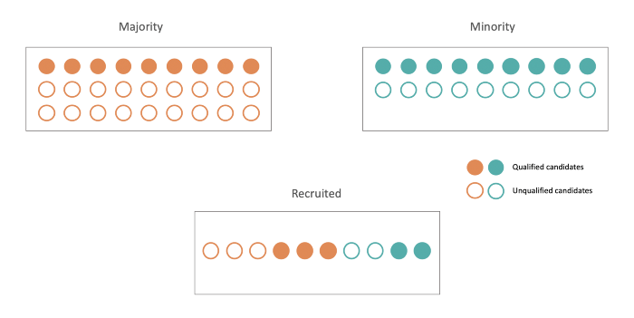
In other words, the probability of attaining the positive outcome is independent of group membership. In practice, courts allow a certain deviation from this standard, perhaps that the disadvantaged group must have a positive classification rate of at least 80% of the advantaged group. This is called the 80% rule.

An example of statistical parity. The applicant pool and group of recruited individuals are both composed of 3/5ths majority applicants. This chart comes from Alexandre Landeau’s blog.

There are many other different (and sometimes incompatible) definitions of fairness. The chapter “Classification” in Fairness and Machine Learning by Barocas, Hardt and Narayanan is a good resource for this.

A running example

We now turn to a running example in the Hu and Kohler-Hausmann paper that helps illustrate the difference between the statistical fairness and causal reasoning approaches. It will also eventually help explain Hu and Kohler-Hausmann’s critique.

Gender discrimination in Berkeley graduate admissions

A study of University of California Berkeley graduate admissions from the 1970’s found that programs accepted 44% of applications from male applicants and only 35% of applications from female applicants. However, when we consider the percentage of men and women accepted to each graduate department individually, the number of female applicants accepted are approximately proportional to the number of female applicants.

As it turns out, there were many more female applicants to humanities graduate programs than science, mathematics and engineering ones. And since the humanities graduate programs are more competitive (their acceptance rates are lower), more women are rejected than men as a proportion of the total pool of graduate applicants, but not within each department.

For a toy example of how this can happen, see the table below of simulated admissions statistics. For the sake of simplicity, there are only two departments, math and history. Although women are accepted at higher rates when each department is considered individually, when they are considered together, women are accepted at a lower rate than men.

	Math		History		Overall
	Men	Women	Men	Women	Men	Women
Applied	40	5	8	6	48	11
Accepted	25	4	1	1	26	5
Percent accepted	63%	80%	13%	17%	54%	45%

This example concerns human, rather than algorithmic, decision making, but Hu and Kohler-Hausmann’s critique applies to both. Kohler-Hausmann has argued elsewhere that U.S. jurisprudence on discrimination misses the mark the same way statistical and causal notions of fairness do.

Making assumptions explicit

How might we evaluate this example under the definition of demographic parity described above? Should we measure demographic parity at the university-wide level or department by department? On the one hand, university departments likely make independent decisions about who they admit to graduate programs, so fairness at the department level seems natural; on the other, it seems objectionable that the overall university admissions place greater burdens on women. The statistical criteria can only get us so far.

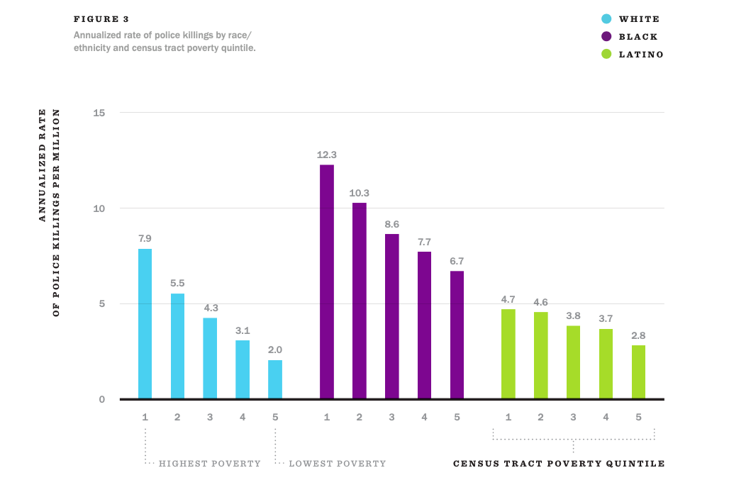
In theory and in practice, there are so many possible explanations for how some set of descriptive statistics came to be that it becomes very difficult to make definitive statements about which factors influenced the outcome. This is the case even when a large body of literature shows robust correlations between membership in a disadvantaged demographic group and adverse outcomes.

Even when there are robust correlations between demographic group membership (in this case race/ethnicity), it is difficult to use statistical measures to definitively determine what factors influence the outcome. Credit to Justin Feldman for the graphic.

The causal reasoning approach, however, tries to disambiguate these different alternatives and properly attribute responsibility to different features influencing the outcome. All that is necessary is to specify a model of how the data is generated. The first step in creating a causal model is enumerating the relevant factors we think might be influencing the outcome and how they influence each other.

One of the reasons why a causal model is able to attribute cause in the first place is the assumption that we can change the relationship between any two features while leaving the other causal relations unchanged — this is called modularity.

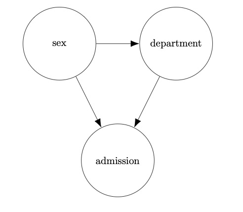
In the Berkeley admissions example, we think the admissions process as being determined by two factors: sex and department choice. Sex may play a “direct” role in admission (if, for example, the admissions committee has a preference for candidates of one sex over another). Sex also has influence over department choice, since a greater proportion of women apply to humanities departments. Finally, department choice has an influence on admission, since departments admit candidates at different rates. This allows us to draw a diagram like the one below:

In this diagram, there are two paths for gender to affect graduate admissions. There is the “direct effect” which would be caused by gender-based preferences on the part of a department, and there is the “indirect effect” caused by the effect of gender of the composition of the applicant pool. (Although the “direct effect” is often the target of anti-discrimination measures, Hu has argued elsewhere that the distinction between direct and indirect effects is largely arbitrary.)

One of the reasons why a causal model is able to attribute cause in the first place is the assumption that we can change the relationship between any two features while leaving the other causal relations unchanged — this is called modularity. This assumption allows us to measure how change in one variable affects others. A fundamental tool of causal reasoning, the do-operator mathematically formalizes this notion. To see how this works, we can use the following example loosely adapted from Ferenc Huszar’s blog:

Let’s say you have a thermometer which reads temperature \(X\) and a true value of the temperature outside \(Y\). The probability distribution of \(Y\) given \(X\), \(\Pr(Y \mid X)\), should be a distribution concentrated near \(X\) with some randomness due to the error in the thermometer reading. By contrast, the interventional conditional probability \(\Pr(Y \mid \texttt{do}(X = x))\) using the do-operator is the probability distribution of \(Y\) given that we set the value of \(X\) to some value \(x\) (say by fixing the thermometer needle to a certain position). Since the thermometer has no causal influence over the actual temperature, this distribution \(\Pr(Y \mid \texttt{do}(X = x))\) would just be equal to \(\Pr(Y)\).

In the Berkeley admissions case, it would be possible to detect the “natural direct effect” of sex on the outcome by comparing the outcomes for \(\texttt{do}(\text{sex}=\text{Male})\) and \(\texttt{do}(\text{sex}=\text{Female})\), or we could manipulate the variables in a number of other ways to isolate the effect of different causal pathways.

A conceptual critique

Hu and Kohler-Hausmann’s objection to the causal reasoning approach is that it makes unsound assumptions about what the social categorization based on sex is and therefore how it affects and is affected by social phenomena. Rather than encompassing just biological or phenotypic features, sex determines salient social categories because of the “web of social relations and meanings” that go along with the biological or phenotypic features. As it relates to the example above, they would argue that that being a woman does not cause a higher likelihood of preference for the humanities; preferences for the humanities partially constitute the social meaning of the group “women”. Of course, there are many other things that contribute to making “women” a salient social group. Consider another example from their paper: Catholicism is characterized by belief in the resurrection of Christ, papal infallibility, and the practice of attending Mass, among other things. Changing any one of these beliefs would influence the meaning of the others. It isn’t necessary that every member of the group adhere to the constitutive features of the group — an individual can still be Catholic without attending Mass every week — but weekly mass is an essential constitutive feature of what defines Catholicism.

They would argue that that being a woman does not cause a higher likelihood of preference for the humanities; preferences for the humanities partially constitute the social meaning of the group “women”.

Why is this important? The techniques of causal reasoning depend on the assumption of modularity, but altering a constitutive feature of a social group changes the meaning of the social group itself, sending out ripple effects to other constitutive features. Under the causal reasoning approach it should be possible to replace “Mass at Church” with “Shabbat at Temple” while still retaining the exact social meaning of Catholicism. Similarly, it should be possible to change women’s graduate departmental preferences without changing the multitude of gendered social phenomena that track women to those departments in the first place. But if women tended to apply to STEM departments, while men tended to apply to humanities departments, the nature of gender categories (and the departments themselves) would be substantially different, leading to changes in other gendered social phenomena. In other words, making modular changes to the meaning of a social group just isn’t possible, so the causal reasoning approach fails. In fact, as Hu and Kohler-Hausmann point out, part of the reason to enact anti-discrimination policy in the first place is to break gendered associations in academic fields, since these gendered associations lead to imbalanced departments and a range of negative downstream effects.

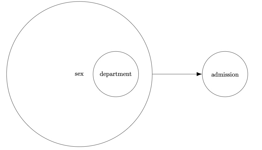
If we were to try to draw a diagram showing the relationships between sex, department and admission under the philosophy described by Hu and Kohler-Hausmann, it might look something like this:

With causal relations, we could ask counterfactual questions, like: “If sex did not play a role in graduate applicants’ department choice, how would admissions statistics for women be different?” But with the constitutive relations, it is no longer possible to ask such clean counterfactual questions, precisely because what it means to be a member of a sex is to have a higher likelihood of being tracked towards certain departments. Thus, to encode fairness into algorithms using Hu and Kohler-Hausmann’s approach, it is no longer possible to use causal counterfactual questions to neutralize causal factors that inappropriately affect the outcome. Instead, it is necessary to come to an understanding of what is owed to different social groups given the various social phenomena that constitute them: what fair treatment between social groups actually means given the statuses and associations attached to demographic groups. And then we must design fairness policies that achieve this.

To conclude

Causal reasoning promises to disambiguate measures of discrimination to help decision makers weigh in on the various explainations for the impact that sensitive attributes may have. However, Hu and Kohler-Hausmann argue that traditional causal reasoning makes unsound assumptions about the nature of social groups. Their work calls for a reimagining of what mathematically formal definitions of fairness can be — and the normative assumptions that underlie them.

The Hu and Kohler-Hausmann paper is available on the arXiv and the FAT* ’20 conference.